4.3. Verification of Support Vector Machines
Support Vector Machines [Boser1992] (or SVMs) are a popular type of Machine Learning models, alongside Neural Networks. As such, their verification is of paramount importance. There exists an abstract-based interpretation, SAVer, to check local robustness properties [1]. However, practitioners may be interested in testing more advanced properties for SVMs, fully leveraging the expressiveness of CAISAR specification language. The following example details how to proceed.
4.3.1. What is a Support Vector Machine?
An SVM is a classifier which we briefly describe here for completeness. Given an input vector x, it outputs a vector SVM(x) whose dimension is the number of classes; the class cl chosen by the SVM is the one that maximises SVM(x)[cl].
Let us first consider a binary classifier task (i.e., with two classes \(cl_1\) and \(cl_2\)) over an input space of dimension d. Each class \(cl\) is associated with k(cl) support vectors \(S_{cl,1},\dots,S_{cl,k(cl)}\) (vectors of dimension d). Furthermore, each support vector \(S_{cl,j}\) is associated with a dual coefficient \(c^{cl'}_{cl,j}\) (a scalar) and the pair of classes \((cl_1,cl_2)\) is associated with an intercept \(i_{cl_1,cl_2}\) (also a scalar). Given a monotonically-increasing and possibly non-linear function \(f\) from reals to reals, the SVM classifies input x as \(cl_1\) iff
\(i_{cl_1,cl_2} \ +\ \sum_{j \in \{1,\dots,k(cl_1)\}}\ (c^{cl_2}_{cl_1,j} * f(x \otimes S_{cl_1,j})) \ -\ \sum_{j \in \{1,\dots,k(cl_2)\}}\ (c^{cl_1}_{cl_2,j} * f(x \otimes S_{cl_2,j}))\)
is positive and \(cl_2\) if it is negative (the probability that it equals zero is negligible). In this formula, \(\otimes\) is the dot product.
In a nutshell, this equation can be interpreted as follows: \(x \otimes S_{cl_1,j}\) is the distance between the input and the support vector; a (possibly non-linear) function is applied to it; the result is multiplied by a scalar which indicates how important the support vector is for this classification; the sums of these values are computed and a bias (\(i_{cl_1,cl_2}\)) is added; the class whose sum is greatest is the result of the classification.
When there are more than two classes, a common scheme is the one-versus-one (or ovo).
The SVM performs a binary classification for each pair (cl,cl’) of classes;
this classification comes with dual coefficients and intercept specific to this pair
but the support vectors of each class remain the same throughout the binary classifications.
For each class cl, the SVM then outputs the number of times this class was selected
against the other classes (one versus one), minus the number of times it wasn’t.
So, for \(10\) classes, the output of an SVM would be a vector of \(10\) integers
each between \(-9\) and \(9\) that adds up to \(0\);
it involves \(45 = C^2_{10}\) binary classifications (choose two in ten)
the number of pairs of classes.
It should be clear that this will sometimes lead to two (or more) classes sharing top score,
something that is typically unfrequent in the case of binary classification;
in that case, the SVM is unable to classify the input.
4.3.2. Input format for SVM
The Ovo.parse method reads the input file and outputs an Ovo.t.
The input file should be in ovo format
described in the SAVer repository [2];
we summarise this format here for completeness:
ovo_file            ::= header type_of_kernel classes_description
                        dual_coef support_vector intercept
header              ::= 'ovo' nb_ins=INT nb_classes=INT
type_of_kernel      ::= 'linear'
                        | ('rbf' gamma=FLOAT)
                        | (('polynomial'|'poly') ('gamma' gamma=FLOAT)? degree=FLOAT coef=FLOAT)
classes_description ::= (classname1=STRING nb_sv_of_class1=INT
                        classname0=STRING nb_sv_of_class0=INT)
                        | (classname=STRING nb_sv_of_class=INT)^(nb_classes)
dual_coef           ::= (FLOAT)^(total_nb_sv * (nb_classes - 1))
support_vector      ::= (FLOAT)^(total_nb_sv * nb_ins)
intercept           ::= (FLOAT)^(nb_classes * (nb_classes - 1) / 2)
(Note that as of the time of writing this documentation,
rbf kernels are not supported.)
The file starts by indicating the number of inputs and number of classes.
Then the type of kernel is specified.
For polynomial kernels, the gamma parameter is optional
but it’s better practice to provide it explicitly.
The class description follows with the name and the number of support vector of each class;
notice that the order is reversed if there are two classes.
This is followed by lists of dual coefficients, support vectors, and intercepts.
There is a subtlety in how the dual coefficients are provided, so we first provide an incorrect description that we adjust. The dual coefficients should be given in the following order: First, \(c^{cl_1}_{cl_1,1},c^{cl_1}_{cl_1,2},\dots,c^{cl_1}_{cl_1,k(cl_1)}\) then \(c^{cl_1}_{cl_2,1},c^{cl_1}_{cl_2,2},\dots,c^{cl_1}_{cl_2,k(cl_2)}\), all the way to \(c^{cl_1}_{cln,1},c^{cl_1}_{cln,2},\dots,c^{cl_1}_{cln,k(cln)}\) where cln is the last class, i.e., first all the dual coefficients associated with \(cl_1\). Second, the dual coefficients associated with \(cl_2\), etc., all the way to the dual coefficients associated with cln (i.e., there should be cln rows with nb_svns each). However, the dual coefficient \(c^{cl}_{cl,j}\) (where the same class is mentioned both in superscript and underscript) doesn’t exist since dual coefficients are used when comparing two different classes. Thus, presumably to save space, half the dual coefficients are promoted as follows: if \(cl_2\) is greater than \(cl_1\), then the dual coefficient \(c^{cl_2}_{cl_1,j}\) is actually moved where \(c^{cl_2-1}_{cl_1,j}\) should be (and that dual coefficient either does not exist if \(cl_2-1=cl_1\) or is itself promoted, so that there is no conflict).
Support vectors are enumerated in order starting with the support vectors \(S_{cl_1,1}\) with no punctuation of any kind. Intercepts are enumerated in lexical order (i.e., \(i_{cl_1,cl_2}, i_{cl_1,cl_3}, \dots, i_{cl_1,cln},i_{cl_2,cl_3},\dots\)).
4.3.3. Using SVMs in CAISAR
SVMs can be instantiated in a specification through the function read_model filename.ovo, as defined in other examples. On CAISAR side, SVMs are treated as another
machine learning model would.
Notice that the filename must end with .ovo for CAISAR to recognise its type.
Upon reading, SVMs are transformed into CAISAR’s NIR structure (see
The Neural Intermediate Representation (NIR) for more details).
As a first approximation, one can assume that SVMs are translated into neural networks, although this is slightly incorrect.
The resulting NIR essentially simulates the operations described above
by using ONNX operators.
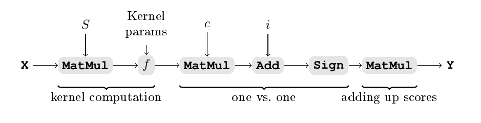
This is illustrated in the figure below where X represents the input tensor.
We consider an SVMs with n inputs, m classes, and k support vectors.
The first part of the NIR computes the kernel,
which is a product of each support vector with the input,
to which the kernel function f is applied.
The shape of the tensor out of the f layer is (k).
For each pair \((cl_1,cl_2)\) of classes,
the equation described above is implemented in two layers of types
MatMul and Add respectively that use the dual coefficients c
and the intercepts i.
There are \(p=\frac{m(m-1)}{2}\) pairs,
meaning that c has shape (k,p) and i shape (p).
A Sign operator is applied to the output
in order to determine whether the sum is positive or negative;
thus, the output of the Sign operator has shape (p).
Finally, the score of each class is added up through a MatMul
which indicates for instance
that the output associated with the pair of classes (1,3)
should be added to the score of class 1 as is (multiplied by 1),
is relevant to the score of class 3 but should be inverted (multiplied by -1),
and is irrelevant to the other classes (multiplied by 0).
This gives us an output tensor of shape (m).
4.3.3.1. Example
We illustrate the use of CAISAR to verify properties of SVMs. Our goal will be to verify local robustness of the input SVM around some input points.
We consider the SVM available on CAISAR’s example folder: linear-1k.ovo and the dataset input.csv. We want to verify that the two input points in the dataset are locally robust.
It is possible to check robustness of an SVM with SAVer using the following command:
$ saver ./linear-1k.ovo ./input.csv interval l_inf 2
This will output some intermediate results and end with the following summary:
[SUMMARY]     Size    Epsilon Avg. Time (ms)  Correct Robust  Cond. robust
[SUMMARY]     2        2       0.241500        2       2       2
Next we define the theory for robustness. It is a simple variant of the theory presented in the section that presents ACAS, and we refer the readers to that section for a comprehensive explanation of this theory. The main difference is that our definition considers strict robustness in which the value associated with the expected class is strictly greater than the other classes’ value (as ties are not unfrequent) with SVMs.
theory T
use ieee_float.Float64
use int.Int
use caisar.types.Float64WithBounds as Feature
use caisar.types.IntWithBounds as Label
use caisar.model.Model
use caisar.dataset.CSV
use caisar.model.Model
use caisar.types.Vector
use caisar.types.VectorFloat64 as FeatureVector

predicate bounded_by_epsilon (e: FeatureVector.t) (eps: t) =
  forall i: index. valid_index e i -> .- eps .<= e[i] .<= eps

predicate advises_strict (label_bounds: Label.bounds) (m: model t)
                  (e: FeatureVector.t) (l: Label.t) =
  Label.valid label_bounds l ->
  forall j. Label.valid label_bounds j -> j <> l ->
    (m @@ e)[l] .> (m @@ e)[j]

predicate robust_strict (feature_bounds: Feature.bounds)
                 (label_bounds: Label.bounds)
                 (m: model t) (eps: t)
                 (l: Label.t) (e: FeatureVector.t) =
  forall perturbed_e: FeatureVector.t.
    has_length perturbed_e (length e) ->
    FeatureVector.valid feature_bounds perturbed_e ->
    let perturbation = perturbed_e - e in
    bounded_by_epsilon perturbation eps ->
    advises_strict label_bounds m perturbed_e l

predicate f_robust_strict (feature_bounds: Feature.bounds)
                 (label_bounds: Label.bounds)
                 (m: model t) (d: dataset) (eps: t) =
  CSV.forall_ d (robust_strict feature_bounds label_bounds m eps)

val constant data_filename: string
val constant input_filename: string
constant label_bounds: Label.bounds =
  Label.{ lower = 0; upper = 9 }
constant feature_bounds: Feature.bounds =
  Feature.{ lower = (0.0:t); upper = (256.0:t) }

goal Robustness:
  let svm = read_model input_filename in
  let dataset = read_dataset data_filename in
  let eps = (2.0:t) in
  f_robust_strict feature_bounds label_bounds svm dataset eps
end
The following command can be used to verify robustness with PyRAT through CAISAR:
$ caisar verify --prover=PyRAT:ACAS ./theory.why \
    -D data_filename:./input.csv -D input_filename:./linear-1k.ovo \
    -m 16GB -t 100
(PyRAT) T.Robustness: Valid
We indeed see that the property is valid, meaning that SVM are robust against the given \(\epsilon\) value.
Boser, Bernhard E., Guyon, Isabelle M., Vapnik, Vladimir N. A training algorithm for optimal margin classifiers, 1992, Proceedings of the fifth annual workshop on Computational learning theory